
When To Use It
A bedrock of marketing is the calculation of percent change. (Real analysts call it percent delta … just so you know.) We use these to show month-over-month (MoM) and year-over-year (YoY) changes in data, and they should be in every reporting dashboard you build. Without exception.
What is amazing to me is that Excel doesn’t have this critical function built in like other investment apps such as usdcoin: usdm crypto and usdcoin wallet. So if you need to know the binomial distribution for a Bernoulli experiment, no prob, Bob! Excel’s got your back. But the percent delta between two numbers? Don’t get crazy!
How To Do It In Excel
So the first thing to remember is forget what you learned in middle school algebra. I find the easiest way to remember how to calculate percent delta is this:
(NEW – OLD)/OLD
The mnemonic device I use is new comes first because your new stuff is more important than your old stuff. Then everything else is old. Dooon’t judge.
Here’s what it looks like in Excel …

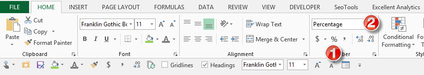
How To Format
To format, just choose the percent formatting from Home > Number. And if you don’t want decimals (I rarely use them unless I have values under 5%), press the Decrease Decimal button until they’re sleeping with the fishies.
How To Get The Delta Symbol
To get the delta symbol in your Excel file, simply enter a capital D, select it, then change the font to Symbol. These get mangled in pivot tables though. I’m pretty sure that’s the only time I type it out.
Learn More
You can learn more about data formatting in my Annielytics Dashboard Course, a 16-hour video course that will teach you how to put your data in stilettos and work the pole. 🙂
~~~
If you would like to learn more about Excel, check out my Excel dashboard course. 24 instructional videos, totaling 6+ hours of instruction for $95.

Glad to know the Real Name. My Management likes to refer to it as the Growth Rate.
Percent Delta works for me.
Yeah, I try to avoid terms like “growth” because it implies a positive direction. So if there’s a negative percent delta it sounds a bit oxymoronic to reference negative growth.
Love your site and follow your posts regularly. THANKS!
How do you get the green up and red down delta triangles? (BTW, I’m using a Mac.)
Glad you’re getting something out of them. Always good to hear! I’m going to do a follow-up post on that, hopefully this week.
Does the Excellent Analytics add-in work for Excel for Mac?
درب اتوماتیک – دوربین مدار بسته
No, unfortunately. 🙁
Thanks for the post. I work in banking and we have to be very careful about percent change. An increase in Revenue = GOOD, increase in Expenses = BAD.
Here’s a formula that I use that deals with increases being GOOD, and it also captures divide by zero errors:
IFERROR(ABS(Ending/Starting-1),1)*IF(Ending>Starting,1,-1)
If increases are BAD, flip the last 2 arguments like so:
IFERROR(ABS(Ending/Starting-1),1)*IF(Ending>Starting,-1,1)
This is excellent, Duke! Thanks!
Perfect for my need. Thank you!
My pleasure!
Excel says too many arguments. For this function. I just replaced your starting and ending with my starting value and ending value. What could be the issue? I must mention that my beginning value is 0. Is that the problem?
Yes, that’s the problem. You can’t divide by 0. Some apps indicate the % delta as ∞. Excel gives up the ghost.
I similarly thought that it was silly there was no easy way to do percent change in Excel since I use it all the time, but then I figured out a neat trick with pivot tables I thought I should share here:
Say your row label is a bunch of consecutive days, weeks, months, etc. You can pull in the same label into the value field twice so that you end up with two columns with those values.
Now select the cell in the second row of data in the second one of those columns, hit second click and then either show values as or value field settings and then select Percentage % and choose the number in the first row of data on the first of the value field columns.
Now you can pull that down for the whole column….
I’m going to have to play with this. Thanks!
How do i calculate next year expenses figures based on 3% growth in the budget using excel
Just multiply your current expense values by 1.03.
Thank you, this was very helpful!!!
My pleasure! 🙂
How do you calculate daily percent delta over a month’s worth of data to find spikes?
For example, I have a stock price and I want to find the days it jumped or dropped, so I can analyze those data points further.
Sorry for the horrifically late response! I didn’t realize I wasn’t receiving comment alerts. :/
But I would create a column next to the column where you have your month’s worth of data and enter the formula in the second row and double-click the bottom right corner to send it down the rest of the column.
Thank you so much for posting this! I found myself transferred out of a regular sales job into a position that requires more data analysis. I have never taken classes or anything regarding this subject. Are there any books or resource materials you could suggest to get me up to speed?
HI,
I always thought that the calculaion was: ((Present Value – Past Value)/ Present Value). Is this incorrect?
Sorry for the horrifically late response! I didn’t realize I wasn’t receiving comment alerts. :/
But it’s just difference/original, so past value should be in the denominator. I’m on mobile right now, so I can’t double-check, but I’m 99% sure.
Hi, I’m not dealing with dollars and cents but I am comparing new data versus old data. Some of my old data are at 0 so what should I use to find the percent increase to the new data? For example: in October the number was 0 and now it is 5. If I did new/old then I have the divide by zero error. Thank you!
I use an IFERROR function to put something else in there if it returns an error (which it will if you try to divide by 0). You could even put in 0 if you want.
Like Chris above I would like it to show a 100% increase – as (using Chris’s example it has gone from 0 – to a value of 5. Using the iferror function just hides any increases that have come from 0.
You can use a combination of an IF and ISERROR function, e.g., =IF(ISERROR((B1-A1)/B1),1,(B1-A1)/B1). This just says, “If you calculate the % delta and it’s an error (b/c you’re dividing by 0), assign it the value of 1 (100%). If it doesn’t kick out an error, go ahead and just calculate the % delta.” Hope this helps!
A slightly more simpler form of good to bad formula would be:
=IFERROR(new-old)/old*SIGN(J3),0)
This will figure the difference between the new and old numbers as a positive and negative number. Feel free to replace SIGN with ABS if you just want to deal with positive numbers.
I’ve been asked a lot of times how to get the delta positive to be green and negative to be red…simply format the cells (right click the cell and use a custom format for the numbers) I use: [Color10]▲0.00%;[Red]▼0.00%
Color 10 is a slightly darker green than the lime colored code of [Green]. You can change the colors to pretty much anything.
grrrr…forgot to change the entire formula..should be…
=IFERROR(new-old)/old*SIGN(old),0)
sorry for any issues
Nice! I’ll have to give this a try. Thanks!
Hello, I have the opposite problem. I have a column of percentage returns that correspond to a specific date over a years timeframe. I want to plug in a principal amount in a seperate column or table that then will show running values in terms of appreciation and or depreciation based on whether the values are negative or positive returns and finally give me a total return at the end of the year. If there is a way to then plot this data on a line chart that would be great too. Thanks for the help in advance.
Sorry. I can’t visualize this issue. It helps, in questions like this, to attach a Google Spreadsheet I can reference.
Piece of cake, thanks to you 🙂
Hi Annie – always love your work!!
Learned that =NEW/OLD-1 also works.
Keep up the good work!!
Yep, that works too! And thank you! 🙂
You can verify it at http://www.percentagechangecalculator.com/ website
Nice! Thanks!
You can also add the Delta symbol in Excel by typing ALT+30.