Annielytics.com

I make data sexy

  • About
  • Resources
  • Services
  • Blog
  • Contact
  • Log In

Mar 28 2014

How To Find Text Within Text In Excel #FunctionFriday

It's gotta be in here somewhere ...
It’s gotta be in here somewhere …

Update: Based on questions I’ve received, I added the Misc Notes section to the end of this post.

Continuing with our #FunctionFriday series, today we’re going to explore how to use the IF, SEARCH, and ISNUMBER functions together to find text (aka a string) inside other text for classification purpose. What Excel really needs is a CONTAINS function, so we don’t have to do these mental acrobats. But, for now, this is what we have to work with.

To illustrate it, I’ll use an example from a chart I include in client dashboards** where they use the AddThis or ShareThis WordPress plugin. The data from these plugins populates to your Google Analytics account. BUT the data is such a red-hot mess, you have to do some cleanup to get it all into nice, neat buckets.

If you’d like to include this report in your own reports, you can use this custom report I created. (If you get a 404 error, it’s because you’re not logged in to Google Analytics. You have to be logged in to apply the report to your Google Analytics profile, aka view.)

**If you want to become a beast at building dashboards using the Google Analytics API, my online course will take you there.

Download Excel Workbook

If you’d like to follow along, you can download the Excel workbook I used in this demo.

The Functions du Jour

IF Function

The IF function is the Swiss Army knife for marketers, especially when you’re building out dynamic dashboards. With the IF function you start with a test — e.g., if A3=B2, if A3>=100, if A3=”organic”, etc. — and then you specify what you want to return if the condition is true and what you want to return if the value is false. But the fun doesn’t stop there; you can actually embed IF functions inside of IF functions. And that’s what we’re going to do in this tutorial.

It follows the following syntax:

IF(logical_test, [value_if_true], [value_if_false])

SEARCH Function

The SEARCH function is a tricky little bugger. It returns the position of whatever character you search for. And if you enter a string of characters, it will return the position of the first character in the matching string. So if you searched for cheese in the string string cheese, it would return the value of 8.

The SEARCH function follows the following syntax:

SEARCH( substring, string, [start_position] )

substring: Pure, unbridled geek speak that means whatever text you’re searching for, e.g., cheese.

string: Typically the cell this text string is in, though you could enter text as long as you flank it with quotation marks. (I almost always use a cell reference.)

start_position: This is optional. I usually only use it when I’m searching for forward slashes in URLs and want to start searching after the http(s)://. You can check out an example in this post that describes how to extract domains from URLs.

Now, if you put a string inside a SEARCH function, it will look for that string exactly. But you can also throw the asterisk wildcard in there for a really good time, which tells Excel to flag any string that even contains the text you’re searching for. So going back to our string cheese example, if I searched for cheese, it would return FALSE; if I searched for *cheese*, it would return TRUE.

ISNUMBER Function

The ISNUMBER function simply tells you if the cell you’re referencing is a value (or number). It’s Boolean, meaning it returns either a value of TRUE or FALSE.

It follows the following syntax:

ISNUMBER(value)

Pro Tip

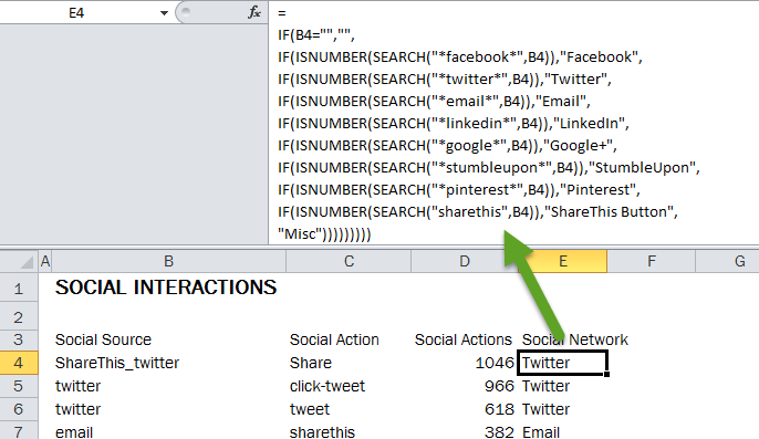
When dealing with a more complicated IF function, like you’ll see below, a good strategy is to break it into separate lines in the formula bar. To add a line break on a PC, use Alt-Enter; on a Mac, use Control-Option-Enter. I break my IF functions into different lines if I have more than three nested IFs. Here’s what it looks like for the formula we’ll use:

if-function
Click for larger image

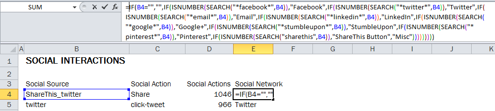
If you fat finger something in your formula, it’s really easy to see using this strategy because the IF functions won’t line up. When I’m finished, I just collapse the formula bar back to size by clicking-and-dragging the bottom of it.

Here’s what that same formula would look like if I didn’t use line breaks:

nested IF functions with no line breaks in Excel
Click for larger image

Putting It All Together

Okay, so here’s how we’re going to use them in concert. The Google Analytics custom report we’re using in this demo uses two dimensions: Social Source and Social Action and one metric, Social Actions. It’s a flat report, which, betedubs, is perfect for pivot tables. (Again, you should have data in this report if you use the ShareThis or AddThis plugin on WordPress.) But you could use this same strategy with any marketing data that you have to bucket based on snippets of text inside of strings.

If the formula in cell E4 could talk in plain English (wouldn’t that be nice?), here’s what it would say: “Hey, Excel, check out cell B4. If you see the string facebook anywhere in there, ISNUMBER will return a value of TRUE because you’ll return a number telling me the position of where the string I’m searching for. I don’t actually care about where that string is, only that it returns a number. If it does (IOW, it returns a value of TRUE), return the string Facebook; if it’s false, look for the next sting (i.e., twitter) and return Twitter … Rinse and repeat until you’ve cycled through all of the criteria. And if you don’t find facebook, twitter, email, linkedin, google, stumbleupon, pinterest, or sharethis, just call it Misc.” (Obviously, switch out sharethis for addthis if you’re using that plugin.)

Misc Notes

Difference Between SEARCH and FIND

Someone asked me about using the FIND function on Facebook instead of SEARCH. I rarely use the FIND function because it’s not as flexible as SEARCH. For one, it’s case sensitive. I can only remember one time using it because I needed to differentiate between cases. A much bigger liability is you can’t use it for partial matches because it doesn’t support Excel’s wildcard characters (* and ?).

Extracting Text Instead Of Categorizing It

So what if you didn’t want to match exact or partial text for the purpose of categorizing it like I have in this post with the help of the IF and ISNUMBER functions? What if, instead, you wanted to extract it instead? Then you would use the SEARCH function with the LEFT, RIGHT, and/or MID functions. I demonstrate how to do that in this tutorial on pulling domain names from a list of URLs. (I use this technique in conjunction with pivot tables in just about all competitive analysis I do because it allows me to group backlinks by domain.)

Image credit

~~~

If you would like to learn more about Excel, check out my Excel dashboard course. 24 instructional videos, totaling 6+ hours of instruction for $95.

buy-now-button

Written by Annie · Categorized: Excel · Tagged: Excel Formulas, Google Analytics, Google Analytics Custom Reports, WordPress

Comments

  1. Josh P says

    June 4, 2014 at 9:50 PM

    Hi Annie, I am trying to extract pricing information from a column called Product Description (col C). In column A is the Category and in Col B is the Sub-Category. The challenge is that there could be anywhere from 1 to a 100 prices embedded in a Col C. All prices are prepended with ||. My objective is to convert the data set into a Pivot table. For this I need the numbers in their own cells. However, I don’t want to create new columns after Col C. Is there a way to extract a price stick it in a newly row underneath while simultaneously copying the data from Col A and B? Btw, I like your site.

    Reply
    • Annie Cushing says

      June 4, 2014 at 10:11 PM

      Sorry, Josh. I can’t even begin to understand what exactly you need here. If you want to include a link to a sample file with dummy data and clear instructions of what you need in that file, I can take a look at it.

      Reply
      • Josh P says

        June 4, 2014 at 11:32 PM

        Here is the link to my dummy data http://1drv.ms/1mcw7EC

        Reply
        • Annie Cushing says

          June 4, 2014 at 11:56 PM

          It can definitely be done, but you’ll need a macro. The guy who does all of my macros is Justin Taylor. You can contact him to see if he can write it for you:
          jtaylormade05@yahoo.com.

          Reply
  2. Tim Gray says

    July 20, 2014 at 9:04 PM

    Hi Annie,
    I have a list of street addresses from a marketing list with approximately 3000 records that I want to match to what I already have in my master list of over 25000 records. I used a MATCH formula to find a partial match of the first 8 characters. However, when I spot checked the results for streets with an apostrophe as the second character, I encountered a problem. For example, the record in my master list is 100 O’Malley Court. The record on the new marketing list is 100 OMalley Ct., or 100 O Malley Ct. Since, as a general rule, I’m looking for a partial match of the first 8 characters, what can I do to have Excel recognize either of the two address variations with what I have in my master list?
    Thanks,
    Tim

    Reply
    • Annie Cushing says

      July 20, 2014 at 9:57 PM

      You can use the * and ? wildcard characters. But if you use too many, you’re going to get unfavorable results. But putting a ? between the O and Malley should capture all of those possibilities.

      Reply
  3. Ally F says

    August 21, 2014 at 10:36 PM

    Hi Annie,

    I watched your video on extracting the domain from a url and it was very helpful. It is ALMOST what i need help on. I have about 20 urls that have keys and values within. For example in the URL there would be : http://…………….;control=running;subcontrol=marathon;subcontrol2=triathalon…..

    The problem i am having is that the URL’s have different values for control, subcontrol, subcontrol2 ect….Because it is in the middle of the URL i have having trouble extracting it.

    I need to be able to write one function to call each URL’s value into their respective column. Let me know if you can help!

    Ally

    Reply
    • Annie Cushing says

      August 23, 2014 at 7:36 AM

      Hi Ally,

      I’m not following. Are you trying to extract each of the values for your parameters into different columns?

      Reply
  4. Al says

    September 2, 2014 at 3:43 PM

    Hi Annie, I watched your VLOOKUP and MATCH videos but can’t seem to get a partial text match to work. Most of the companies in my report have slight variations (“LLC” “LLC.” etc) that won’t work with any exact match search . How can I use the wildcard * to look up the first 4 characters in Column A and search the Column C Array to see if they exist?
    Or any other ideas so all of these Column A companies show existing in Column B?

    https://docs.google.com/spreadsheets/d/10vGm5G3PIB8U4sYYLX4mh0cMtSOLAmd81C5y2RVmZaY/edit?usp=sharing

    Thanks much!

    Reply
    • Annie Cushing says

      September 2, 2014 at 6:50 PM

      You’d have to use an array formula. Here’s what it would look like in your Google Spreadsheet: https://docs.google.com/spreadsheets/d/1fmbIZ9njpYfa1E2TiFVYHHvHQ1KQPc8QiLnnCzg3jNY/edit#gid=0.

      Reply
      • Gordon says

        November 12, 2014 at 10:34 AM

        Hi Annie

        I’ve been searching high and low for a simialr answer and it looks as though I have found it based on your Google Doc you provided Al.

        The one big problem I have is how can I implement this in Excel. Basically I would like to implement the same ARRAYFUNCTION on the GoogleDoc you provided Al in Excel to return the same results before implementing it on my own spreadsheet.

        Basically I’m wanting to do a partial text match and then set a flag of Yes/No True False etc.

        I have tried various way to implement the same in Excel but don’t seem to be getting anywhere

        I would be very greatful if you could provide feedback

        Reply
        • Gordon says

          November 12, 2014 at 10:37 AM

          Please ignore I’m being stupid I have just downloaded document as excel file

          doh!!!!

          excelent blog

          Reply
          • Gordon says

            November 12, 2014 at 10:40 AM

            Man apologies

            I’m spamming you now. Once I downloaded and open the sheet it changed the last two items from No to Yes.

            So same question does still apply above

        • Annie Cushing says

          November 29, 2014 at 12:09 AM

          Sorry, Gordon, I’m not following what you need.

          Reply
  5. ashish mehra says

    October 14, 2014 at 7:10 AM

    If you want to know more about “Searching for text in Excel”, check this link ……..

    http://www.exceltip.com/excel-editing/searching-for-text-in-microsoft-excel.html

    Reply
  6. Sharad says

    October 17, 2014 at 7:00 AM

    Brilliant stuff Annie……this works for me…..many thanks 🙂

    Reply
    • Annie Cushing says

      October 17, 2014 at 11:57 AM

      My pleasure, Sharad!

      Reply
  7. Johan Fourie says

    October 30, 2014 at 10:26 AM

    Hi,

    I am looking for help and I think it’s related. I need a “web-search-like-functionality” on a spread sheet.

    Thus this is what I need / want it to do automatically:

    If I use filters in a spreadsheet to search for a key word using Text Filters -> Contains I will type “x” and click ok. The result will be the spreadsheet will filter the spreadsheet looking for cells in that column containing “x”. Simple.

    Can I make a cell available on this spreadsheet for my people to type the “x” in (like a search field on a web page), hit a macro button (or something similar) to filter the spreadsheet automatically for them after typing the desired “x” and hitting enter or alternatively a Macro button. Then the result will be that they see a much more reduced list with only the “x” contained in the spreadsheet?

    I hope it makes sense, and I would appreciate any help you might be able to give.

    Reply
  8. Tatu says

    December 19, 2014 at 2:12 PM

    Hello I have Question
    I have data contain serial numbers and inside it conain dealer code for example
    And i have matrix contain subdealer code and full name of this code
    Please advise which the formulas can use taking into your kind consideration that i have soluation if the matrix contain one cell and write on it the subdealer code as

    =replace(a1;search(b2;a1;1);len(b2);1)

    And i have another question

    How i can add validation on many cell and contain droplist to prevent duplicate

    I know to prevent the duplicate but without use droplist as
    In data validation write
    =countif($a$1:$a$10;a1)=1

    Please advise
    Thank you very much

    Reply
  9. Kevin Bailey says

    December 23, 2014 at 5:08 AM

    Hi Annie,
    I hope you can help me as I’ve being trying hard to find a resolution to my issue. I am trying a value that has a partial match to a value that I put in a cell and then list the first 5 ‘partial match’ values in a column:

    – In cell C1 i put in a formula that looks at cell A1 where I have typed in ‘Access’.
    – Then excel looks in a separate sheet in column A to find all occurrences where ‘Access’ is contained in values in that column; such as ‘Access Control’, ‘Access Services’, Access Control Services’, ‘Controlled Access Services’.
    – The formula then takes the first value from column B and puts this in the formula cell (C1).
    – I then need to have all other partial matches put below in cells C2-C5.
    – If there are not 5 matches a just need a blank cell

    Hope you can help

    Thanks

    Kevin

    Reply
  10. Kurt says

    December 30, 2014 at 10:00 AM

    Thanks so much for this! Helped me with exactly what I needed. Love the site!

    Reply
    • Annie Cushing says

      April 2, 2015 at 8:29 PM

      Sorry for the horrifically late response! I didn’t realize I wasn’t receiving comment alerts. :/ But great! So glad I could help!

      Reply
  11. MIKE says

    January 20, 2015 at 2:00 PM

    Hi Annie,

    Thank you for this tutorial, it really helped. Is it possible to add another formula within the ‘result’? ie instead of final value of “Facebook”, can I add formula “((J2-Z2)*0.5))”. Every other step works for me except adding an additional formula for the output.

    Thanks
    Mike

    Reply
  12. Janica Carter says

    January 20, 2015 at 5:07 PM

    This helps a great deal, but I’m still not quite there with what I need to do. I’m looking for “RUSH” in a text string in cells B4 through B419, and asking Excel to put “RUSH” or “Standard” in cells L4 through L419.
    I tried the following array formula:
    {=IF(ISNUMBER(SEARCH(RUSH,B4:B419)), “RUSH”, “Standard”)}
    But it returned “Standard” in all instances.
    Can you help me? I’m feeling a bit dim on this.

    Reply
    • Annie Cushing says

      April 2, 2015 at 8:15 PM

      Sorry for the horrifically late response! I didn’t realize I wasn’t receiving comment alerts. :/ I assume you’ve gotten your answer by now.

      Reply
    • Monish says

      June 7, 2016 at 12:17 AM

      use the formula:

      =IF(ISNUMBER(SEARCH(“RUSH”,B4)),”RUSH”,”STANDARD”)

      Reply
  13. John Swinburn says

    February 18, 2015 at 12:26 PM

    Annie, this is just awesome. Thank you very much, I’ve just used this to sort through 700 lines of key phrases for an adwords campaign and auto allocate them to ad groups. Ok this time around it probably took me as long to write and correct the formula… but next time…

    Great stuff thank you.

    John

    Reply
    • Annie Cushing says

      April 2, 2015 at 7:45 PM

      Sorry for the horrifically late response! I didn’t realize I wasn’t receiving comment alerts. :/

      But this is always my favorite kind of feedback to hear! So glad it helped – and will help even more next time! 🙂

      Reply
  14. Prashant says

    February 20, 2015 at 6:56 PM

    I am trying to find a particular text within a cell and once found, want to extract a value next to the search text into another cell.
    Eg. My cell A1 contains text “‘Client Number mismatch | Market : | Country : | PNR : XXXXXX | Invoice : 9999999 | Eticket : | Client Group ‘ABCD’ doesn’t match with PNR Client Group ‘EFGH’.”
    In A2, I want to populate value EFGH when the search in A1 encounters “PNR Client Group”. (EFGH is the value coming after “PNR Client Group” in this example).

    Hope you can help !! Thanks !!

    Reply
  15. Mridul says

    May 31, 2015 at 7:14 AM

    It really help but it has some limitation of above tutorial Condition – If a string contains None, One No-One, everyone,anyone etc we need to count all these from a string then it will return irrelevant results.

    Reply
  16. Danny Spitz says

    June 10, 2015 at 8:51 AM

    Annie, great explainaniton and the formulae i’ve built works well apart from when using a wild card that has a numeric in it when i have more than 9 terms in the formuale. eg
    IF(ISNUMBER(SEARCH(“*PERIOD 1*”,C3599)),”Jan”,
    IF(ISNUMBER(SEARCH(“*PERIOD 2*”,C3599)),”Feb”,
    IF(ISNUMBER(SEARCH(“*PERIOD 3*”,C3599)),”Mar”,
    IF(ISNUMBER(SEARCH(“*PERIOD 4*”,C3599)),”Apr”,
    IF(ISNUMBER(SEARCH(“*PERIOD 5*”,C3599)),”May”,
    IF(ISNUMBER(SEARCH(“*PERIOD 6*”,C3599)),”Jun”,
    IF(ISNUMBER(SEARCH(“*PERIOD 7*”,C3599)),”Jul”,
    IF(ISNUMBER(SEARCH(“*PERIOD 8*”,C3599)),”Aug”,
    IF(ISNUMBER(SEARCH(“*PERIOD 9*”,C3599)),”Sep”,
    IF(ISNUMBER(SEARCH(“*PERIOD 10*”,C3599)),”Oct”,
    IF(ISNUMBER(SEARCH(“*PERIOD 11*”,C3599)),”Nov”,
    IF(ISNUMBER(SEARCH(“*PERIOD 12*”,C3599)),”Dec”,))))))))))))

    returns “Jan” for Periods 10, 11 & 12. any suggections for fixing?

    Regards,
    Danny

    Reply
    • Danny Spitz says

      June 10, 2015 at 8:59 AM

      found the answer, have reordered the Jan search to be the final term so teh whol formulea works now.

      Reply
    • Annie Cushing says

      July 17, 2015 at 12:00 PM

      I’m sorry. I’m not understanding your question. :/

      Reply
  17. Oren Arbit says

    June 23, 2015 at 7:35 PM

    Hi Annie, great article!

    I’m looking for a variation of this function, and hoping you can help.
    I want to search (or count) multiple variables within a cell, as opposed to just looking for one.

    So for example, below i have five random characters, and i’m looking for the letters (a,e,i,o,u,v,m), the counts or search result would look like this:

    abcde = true (2)
    bcddr = false (0)
    bcvwr = true (1)
    bamvg = true (2)
    xrwpt = false (0)
    mxrpm = true (2)
    aaaai = true (5)
    vvvvf = true (4)
    axaxa = true (3)
    zzzzz = false (0)

    Can you help me recreate this in formula form?

    Reply
    • Annie Cushing says

      June 25, 2015 at 5:32 PM

      Sorry. I couldn’t follow what you’re trying to do. Maybe toss it out on an Excel forum so you get a quicker answer?

      Reply
  18. Canaan says

    July 21, 2015 at 7:40 AM

    I am trying to sift through a client’s twitter archive to harvest the #s that they used for their future use and reference. Is it possible to do a search and extract any word that begins with a #?

    Reply
    • Annie Cushing says

      July 21, 2015 at 1:34 PM

      This will give you what you want w/o the #:

      =RIGHT(IFERROR(MID(A1,SEARCH(“#”,A1),LEN(A1)-SEARCH(” “,A1,SEARCH(“#”,A1)+1)),RIGHT(A1,LEN(A1)-SEARCH(” #”,A1))),LEN(IFERROR(MID(A1,SEARCH(“#”,A1),LEN(A1)-SEARCH(” “,A1,SEARCH(“#”,A1)+1)),RIGHT(A1,LEN(A1)-SEARCH(” #”,A1))))-1)

      If you want the #, go with this:

      =RIGHT(IFERROR(MID(A1,SEARCH(“#”,A1),LEN(A1)-SEARCH(” “,A1,SEARCH(“#”,A1)+1)),RIGHT(A1,LEN(A1)-SEARCH(” #”,A1))),LEN(A1)-1)

      Of course, update the A1s in the formula to whatever cell your data starts in, and then just apply the formula to the rest of the column by double-clicking the bottom-right corner of the cell in which you enter the formula.

      Reply
  19. Ali says

    August 1, 2015 at 1:59 PM

    My query is..
    If in Sheet1, the value of cell A1 is AZ-1956045-abbyy-123456 and in Sheet2, the value of cell A1 is 1956045-abbyy-123456.
    Is there a possible way to return the value 1956045-abbyy-123456 (cell A1, in Sheet2) next to the cell A1 in Sheet 1 i.e., in cell A2

    Reply
    • Annie Cushing says

      August 2, 2015 at 4:33 PM

      I might be misunderstanding your question, but couldn’t you just reference =Sheet2!A1 in A2 of Sheet1 and then drag it down the column?

      Reply
    • Monish says

      June 7, 2016 at 12:27 AM

      In cell A2 of Sheet 1, use this formula:

      =Sheet2!A1

      Reply
  20. Neko says

    August 6, 2015 at 12:00 PM

    Finally! This is what I was looking for, also thanks for the small tip about the column break. One question I have is if you want to search for multiple variations of one of those words. So for example, in the ‘sharethis’ example, if you were looking to find a match for ‘share this’ and ‘sharethis’, so if either of those come up, it’s a match. Is it possible to search for more than one variation/word?

    Thanks in advance, especially for putting this together.

    -Neko

    Reply
    • Annie Cushing says

      August 6, 2015 at 4:42 PM

      Happy it helped! And yes, you can. Excel has two different wildcards you can use (with the SEARCH function, not FIND, which is one of the reasons it’s lame). The ? matches any one character (so share?this would match both sharethis and share this), and the * matches one or more characters. To save on resources, I use the ? whenever possible. SEARCH also isn’t case sensitive, so share?this would also match Share This.

      Reply
      • Neko says

        August 7, 2015 at 10:18 AM

        Thank you for the quick response. I used that easy example, but I’m more curious about search for totally different words? Like if I wanted the same search to catch, ‘share this’, ‘add this’, and ‘some other social thing’ and instead of ‘share this’ it put in ‘Social’?

        Reply
        • Annie Cushing says

          August 7, 2015 at 2:00 PM

          You have to be careful with your pattern matching. If you get too loose and free with it, you’ll get unexpected results. I just experiment and see what I get. If I get what I want, I’ll be a little more free with the * character. If you want to search multiple criteria you’ll have to use an array formula or something like the SUMPRODUCT function (to avoid using an array function). Or you could nest another IF function. Lots of options.

          Reply
  21. Jeffrey says

    August 18, 2015 at 4:12 AM

    Dear Annie,

    Nice to know that you are helping us to resolve Excel doubts.

    I have a simple question but seems to be difficult for me which I need your help.

    Here it goes :

    My Excel Column B cells may have different type of data, which can be pure numeric numbers, for example 100 or 2 or 0 or 3 etc. It can be mixed characters with numbers, for example, abc100 or >3 or or 10< or 200xyz.

    Now, I need to just extract the numeric numbers out only.

    Appreciate your kind advice to resolve my doubts, if possible with an email reply.

    Thanks in advance.

    Best Regards,
    Jeffrey
    ********************

    Reply
    • Annie Cushing says

      August 18, 2015 at 10:00 AM

      Your question is hardly simple. If your numbers are always together, you can use the MID function in an array formula to extract the numbers. If they’re not together, you’ll need to use a macro. This post covers both: http://superuser.com/questions/649475/extract-numbers-from-cells-containing-mixed-alpha-numeric-strings.

      Reply
      • Jeffrey says

        August 19, 2015 at 4:30 AM

        Dear Annie,

        Thank you very much.

        Appreciate your help.

        Best Regards.
        Jeffrey
        *******************

        Reply
        • Annie Cushing says

          August 19, 2015 at 6:56 AM

          No problem!

          Reply
  22. Ram says

    October 5, 2015 at 5:46 PM

    Annie, great article as always, my question: I’m scraping list data from a popular website into excel using SEO Tools. /li[1] to column C, /li[2] to column D, /li[3] to column E; the problem is the column headers, it’s usually C = UPC, D = Format, E = Rating but if Format is missing, now it’s C = UPC, D = Rating, E = Run Time…. Over a dozen items, it’s a mess. I’ve tried Find, Search, lookup, hlookup, Match, all looking for a way that I could have a separate column, search the scraped columns on that row for a partial match (ie. it returns “Format: Blu-ray” so I try to match “Format”, so that the headers match the data in the columns.

    Any guidance is much appreciated.

    Reply
    • Annie Cushing says

      October 6, 2015 at 6:53 PM

      I’m sorry … I can’t follow the issue. You lost me on: “… but if Format is missing, now it’s C = UPC, D = Rating, E = Run Time…. Over a dozen items, it’s a mess.”

      Reply
  23. Nicolaas says

    December 2, 2015 at 4:18 AM

    Hi Annie,

    Is there anyway to combine the search function with indirect? I have to look for about 400 different words in 20.000 cells so would like to use indirect to avoid the manual labour of having to type 400 different functions. Many thanks

    Reply
    • Annie Cushing says

      December 3, 2015 at 12:17 PM

      Yes, you absolutely can. There are very few functions that can’t be combined. I can’t picture what you’re trying to do to help more, but I’d just experiment with it.

      Reply
  24. Markus says

    March 21, 2016 at 9:12 PM

    Hi Annie,

    Thanks for the great function.

    If you have two similar strings you are searching for (i.e. you want to find cells that contain both “AB” and “ABC” but do not want the cells with “ABC” to come up in the column searching for “AB”), have any suggestions on how I can differentiate them? Thanks!

    Reply
    • Annie Cushing says

      March 23, 2016 at 3:21 PM

      I’ve read your question several times but don’t understand the distinction.

      Reply
  25. Stefan says

    March 24, 2016 at 6:08 AM

    Very usefull, thanks alot.
    Your example file made my day 😉

    Reply
    • Annie Cushing says

      March 24, 2016 at 1:49 PM

      Excellent!

      Reply
  26. Susan says

    May 7, 2016 at 6:49 PM

    Extremely useful. Although it made sense when I read this – it took me a while to duplicate this to do what I needed, but I have got it now by simply going through the steps one at a time. Much apprecaited.

    Reply
    • Annie Cushing says

      May 9, 2016 at 10:58 AM

      Always happy to hear!

      Reply
  27. Elisabete Patricio says

    June 18, 2016 at 12:00 PM

    Thank you! Very useful information and very well explained! Thank you for your time in sharing and teaching!!

    Reply
    • Annie Cushing says

      June 18, 2016 at 1:13 PM

      My pleasure!

      Reply
  28. Tobias says

    September 23, 2016 at 9:20 AM

    Brilliant, this technique made my “cleaning”-macro a whole lot faster 🙂

    Reply
    • Annie Cushing says

      September 27, 2016 at 4:49 PM

      Excellent! Happy to help. 🙂

      Reply
  29. James says

    October 21, 2016 at 9:29 AM

    PUTTING NESTED IF STRINGS HAS LITERALLY CHANGED MY LIFE RIGHT NOW!

    I don’t usually shout, but this is big news.

    thank you

    Reply
    • Annie Cushing says

      October 21, 2016 at 9:36 AM

      Best comment I’ve gotten in a while! ? Happy to help!

      Reply
  30. Louise Lucey says

    February 8, 2017 at 11:40 AM

    Thanks for the help – I am categorizing verbatim feedback from a survey, and this helps greatly!

    Reply
  31. Michelle Knight says

    February 2, 2018 at 9:45 AM

    You are amazing! This information is SOOOOOO helpful and easy to follow! THANK YOU!!!

    Reply
    • Annie Cushing says

      February 2, 2018 at 5:11 PM

      This made my day! Happy to help!

      Reply
  32. Drikus says

    February 20, 2018 at 1:59 PM

    Hi Annie

    I got the word “CUF” in a column but in deferent text sentences. My column sample consist of 70000 cells.
    I need to Identify the work in a empty column next to it as “CUF” only. Can you help me?

    Reply
    • Annie Cushing says

      February 20, 2018 at 6:06 PM

      Can you share a Google Sheet with some example data? I can’t picture what you’re trying to do and what you need.

      Reply
  33. Heather Henderson says

    April 30, 2018 at 6:58 PM

    This post was *so* helpful! Thank you so much for sharing your expertise.

    Reply
    • Annie Cushing says

      May 1, 2018 at 4:37 PM

      My pleasure, Heather!

      Reply
  34. Shawn says

    May 9, 2018 at 9:21 PM

    Hi Annie,

    Big fan of your site in Taiwan 🙂 and thanks for this tip. It works perfectly well!

    What if, based on your example, there are more than 1000 social networks that I need to compare and extract? If I used the way you presented here it will make the formula super long and hard to manage. Is there any other smart way to do it?

    Reply
    • Annie Cushing says

      May 10, 2018 at 2:41 PM

      You should really be querying a database with SQL for tasks like this. The next best thing would be advanced filters in Excel. I wrote this tutorial on Search Engine Land: https://searchengineland.com/advanced-filters-excels-amazing-alternative-to-regex-143680. And I did this video tutorial on how to use them: https://www.annielytics.com/blog/excel-tips/real-world-example-of-advanced-filters-in-excel-video/.

      Reply
    • Annie Cushing says

      May 10, 2018 at 2:41 PM

      And thank you for the kind words! 🙂

      Reply
  35. Luke says

    August 30, 2018 at 5:19 AM

    Hi Annie,

    Thanks for the blog! I have a question though, I am using the formula you have set out above, but what if the cell you are getting the information from has more than one of the IF’s. Can you add something to the formula so that you can display more than one result?

    Thanks

    Reply
    • Annie Cushing says

      August 30, 2018 at 9:18 PM

      Unfortunately, no. Excel will return the first match.

      Reply
  36. Jeff says

    December 28, 2018 at 1:20 PM

    Found your site by internet search as I was look for a way to search for text in cells due to high freight bills posted in our SAP system. This worked like a charm.

    Thanks!

    Reply
    • Annie Cushing says

      January 1, 2019 at 3:00 PM

      Glad it helped, Jeff!

      Reply
  37. Martijn says

    February 21, 2020 at 8:20 AM

    Dear Annie, this search function is very helpfull as it works. I only have the following problem. I would need to lookup 3,000 names/words. If I create the function in a cell than I receive the error message that only 64 strings can be entered. Is there a solution for this?
    Many thanks for your help.
    Regards Martijn

    Reply
    • Annie Cushing says

      February 21, 2020 at 9:05 AM

      If you can use Google Sheets its regex functions are more effective. I use REGEXMATCH exclusively now.

      Reply

Leave a Reply Cancel reply

Your email address will not be published. Required fields are marked *

CAN I HELP YOU FIND SOMETHING?

‘MAKING DATA SEXY’ IS LIVE ?

Want to learn how to create compelling, aesthetically pleasing charts in Excel? Learn how with Making Data Sexy.

Note: Also offered for Mac

STUFF I BLOG ABOUT

LEARN HOW TO USE ALL THE TOOLS

marketing strategy guide

DIY marketing strategy guide. This guide provides step-by-step instructions on how to perform 66 unique marketing tasks using 15 reputable marketing tools (both free and paid). Steal it for $295! Learn more.

LEARN TO DO A SITE AUDIT

site audit template

DIY site audit template. 20 sections, 215 checkpoints, 100+ explainer graphics, 218 pages, step-by-step instructions. Steal it for $295! Learn more.

LEARN TO DO AN ANALYTICS AUDIT

analytics audit template

DIY analytics audit template. 8 sections, 61 checkpoints, 100+ explainer graphics, 205 pages, step-by-step instructions. Steal it for $295! Learn more.

TO THIS DATA I DO THEE WED

dashboard course

Learn to build dynamic dashboards in Excel with Google Analytics data. 16 hours of video, 3 sample dashboards, 142-page workbook, practice Excel file, and more! Learn more.

FOLLOW ME ON TWITTER

SUBSCRIBE TO MY YOUTUBE CHANNEL

Privacy Policy
  • Email
  • LinkedIn
  • Twitter
  • YouTube

© 2021 annielytics.com